The isomorphous differences between the native and a derivative dataset can be used to make an isomorphous difference Patterson map. This can be used to locate the heavy atoms manually if there are only a few sites (1 or 2 should be possible). Sometimes, there are more sites than this. A large number of sites necessitates the use of automatic site location methods. Whichever method is used, it is useful to calculate and check the Patterson map first. The Patterson map is calculated with the CNS task file patterson_map.inp.
cns_solve < patterson_map.inp > patterson_map.out [15 seconds]
The output of the patterson_map.inp task file is a CNS binary map for each of the Harker sections. These Harker sections will be determined automatically by CNS, but are currently limited to those sections which are parallel to unit cell axes (diagonal sections will not be written). The Harker sections can be converted to a Postscript image using the command plot_patterson. This takes interactive input from the terminal:
unix% plot_patterson
patterson map file -> patterson_map_y.map
patterson plane (x/y/z) -> y
postscript plot file [patterson.ps]-> patterson_map_y.ps
minimum contour level [2.0]->
contour increment [0.5]->
plot scale factor [0.06]->
plot title -> Experimental Patterson map Y-section
It is important to note that the CNS Harker sections are written out in binary format. Therefore, plot_patterson must be run on the same type of machine as the patterson_map.inp task file was also run.
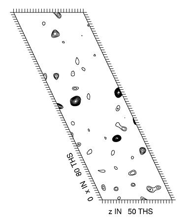
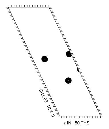
In the example used here the space group is C2 so there is only one Harker section (at Y=0). This is calculated using the native amplitudes and a uranyl derivative. The Harker section shows peaks due to the heavy atoms which are present in the derivatized crystal. Below are the Patterson maps calculated from the experimental data (top), and from the known locations of 3 heavy atom sites (bottom). These sites were located using automatic methods (see the other tutorials for details). The command to calculate the Patterson map from the known locations of the sites is:
cns_solve < predict_patterson.inp > predict_patterson.out [7 seconds]
Again, the plot_patterson command is used to convert the Harker sections to a Postscript image:
unix% plot_patterson
patterson map file -> predict_patterson_y.map
patterson plane (x/y/z) -> y
postscript plot file [patterson.ps]-> predict_patterson_y.ps
minimum contour level [2.0]->
contour increment [0.5]->
plot scale factor [0.06]->
plot title -> Predicted Patterson map Y-section
 |
| Experimental Patterson |
 |
| Predicted Patterson |