The hemihedral twinning is directly incorporated into the refinement target - ie. the data are not detwinned. The least squares crystallographic target used is:
target = ( Fo - k( sqrt [(1-alpha)Fc^2 + (alpha)Fc'^2] ) )^2
where alpha is the twinning fraction (between 0 and 0.5) and Fc' denotes application of the twinning operator. The scale factor k between observed and calculated data remains fixed during a refinement cycle and is only recalculated when the value for the weight between crystallographic and geometric terms is updated. The twinning fraction alpha also remains fixed during refinement. Note that only hemihedral (2-fold) twinning is currently permitted.
The structure used in this tutorial is that of a double mutant (D97A,E99A) of the general diffusion porin from Rhodopseudomonas blastica (B.Schmid, L.Maveyraud, M.Kromer, G.E.Schulz "Porin mutants with new channel properties", Protein Science 7, 1603-1611). The deposited refined model (7prn) and the structure factors (r7prnsf) were obtained directly from the Protein Data Bank. The twinning of the data had previously been identified (T.O.Yeates, B.C.Fam "Protein crystals and their evil twins", Structure 7, 25-29). Comparison of the original model and that after refinement with the twinning included shows negligible changes in the protein structure.
This structure has been previously refined against the data without the twinning taken into account. Therefore, the refinement is begun with simulated annealing using torsion angle dynamics, to remove the bias to the original test set (and improve the model if possible). The use of torsion angle dynamics reduces the number of parameters being refined and hence reduces the degree of overfitting of the data. For an initial model with relatively large errors (due to manual building or misplaced atoms) a starting temperature of 5000K is recommended. In order to decrease the computational time required the colling rate can be increased from 25K to 50K. The simulated annealing refinement task file includes energy minimization both before and after the simulated annealing. Multiple refinement trials can be performed, each with different initial velocities for the molecular dynamics. It can be useful to run 5 or 10 trials if the there are some serious errors in the model - greater variation is usually seen in these areas. The structure factors from the multiple models can also be averaged to reduce the noise in the electron density maps (see the CNS task file optimize_average.inp). The simulated annealing refinement is performed with the CNS task file anneal_twin.inp:
cns_solve < anneal_twin.inp > anneal_twin.out [90 minutes]
The result of the refinement is a new coordinate file (anneal_twin_1.pdb). In the majority of CNS refinement task files information about the refinement procedure is written out at the top of the output coordinate file (as REMARK statements):
REMARK coordinates from twinned data simulated annealing refinement
REMARK twinning operator= h,-h-k,-l  twinning fraction= 0.304
REMARK refinement resolution: 500.0 - 2.25 A
REMARK starting twinned r= 0.1981 twinned free_r= 0.2060
REMARK final    twinned r= 0.1854 twinned free_r= 0.2296
REMARK rmsd bonds= 0.008430  rmsd angles=  1.37200
REMARK wa_initial= 256191  wa_dynamics= 271428  wa_final= 273771
REMARK target= twin_lsq  md-method= torsion  annealing schedule= slowcool
REMARK starting temperature= 2500  total md steps= 100 * 6
REMARK sg= R3 a= 104.400 b= 104.400 c= 124.250 alpha= 90 beta= 90 gamma= 120
REMARK parameter file 1  : CNS_TOPPAR:protein_rep.param
REMARK molecular structure file: porin.mtf
REMARK input coordinates: porin.pdb
REMARK reflection file= porin.cv
REMARK ncs= none
REMARK B-correction resolution: 6.0 - 2.25
REMARK initial B-factor correction applied to fobs :
REMARK   B11=  -1.682 B22=  -1.682 B33=   3.363
REMARK   B12=  -2.765 B13=   0.000 B23=   0.000
REMARK B-factor correction applied to coordinate array B:    6.895
REMARK bulk solvent: density level= 0.371276 e/A^3, B-factor= 41.6062 A^2
REMARK reflections with |Fobs|/sigma_F < 0.0 rejected
REMARK reflections with |Fobs| > 10000 * rms(Fobs) rejected
REMARK reflections with |Fobs|[h,-h-k,-l] = 0 rejected
REMARK theoretical total number of refl. in resol. range:     23999 ( 100.0 % )
REMARK number of unobserved reflections (no entry or |F|=0):     66 (   0.3 % )
REMARK number of reflections rejected:                           43 (   0.2 % )
REMARK total number of reflections used:                      23890 (  99.5 % )
REMARK number of reflections in working set:                  21695 (  90.4 % )
REMARK number of reflections in test set:                      2195 (   9.1 % )
CRYST1  104.400  104.400  124.250  90.00  90.00 120.00 R 3
REMARK FILENAME="/tmp_mnt/Net/franklin/u0/pvm/tmp/porin/twin/anneal_twin_1.pd"
REMARK DATE:24-Jun-99  12:55:09       created by user: paul
REMARK VERSION:0.5
ATOM      1  CB  MET A   1       9.241  57.460  19.295  1.00 26.90      A
ATOM      2  CG  MET A   1       7.910  56.758  18.961  1.00 26.90      A
This information provides a summary of the refinement and also a record of the input data and parameters used to generate this structure.
There is an increase in the free R-value because this model has previously been refined against a different test set, and the annealing serves to remove the bias to this old test set.
The initial model has the same B-factor for all atoms. In order to take account of the possible variation in B-factors throughout the model, individual atomic B-factors are then refined. The B-factors are restrained such that atoms bonded together have similar B-factors. The individual, restrained B-factor refinement is performed with the CNS task file bindividual_twin.inp:
cns_solve < bindividual_twin.inp > bindividual_twin.out [4 minutes]
After this refinement the twinned free R-value is 20.3% and the twinned R-value is 16.3%. The next step is to locate the water molecules which can be seen in a gradient map. The is gradient map is calculated using the CNS task file model_map_twin.nip:
cns_solve < model_map_twin.inp > model_map_twin.out [1.5 minutes]
If you have mapman installed, you can use the command
map_to_omap *.map
to convert the CNS maps to a format which can be read into
O. In O, enter @omac to read in the current
model and map.
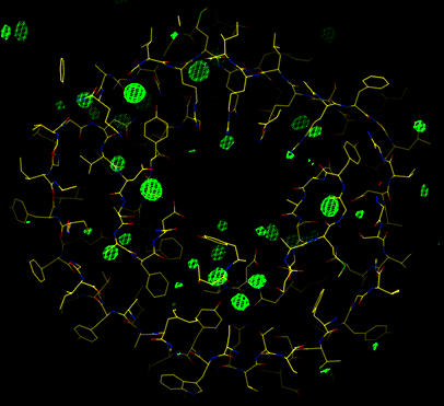
The electron density map clearly shows many water molecules (or possibly ions). The advantage of the gradient map is that it does not require that the data be detwinned prior to map calculation.
 |
| Gradient map (at 4 sigma). |