In this tutorial, MAD phases (see previous tutorial) are improved by solvent flipping and density truncation. In a preliminary step, the solvent content is estimated by using matthews_coef.inp.
cns_solve < matthews_coef.inp > matthews_coef.out [< 1 second]
The estimated solvent content shown in matthews_coef.list is between 0.53 and 0.55. density_modify.inp is modified accordingly by setting the solvent content parameter to 0.54.
cns_solve < density_modify.inp > density_modify.out [27 minutes]
The resulting output files are:
      density_modify.list - listing file with statistics for
                            each modification cycle
      density_modify.hkl  - reflection file with new Hendrickson-Lattman
                            coefficients
      density_modify.map  - map file with modified electron density
      density_modify.mask - file with definition of solvent mask
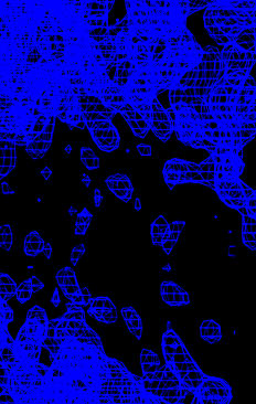
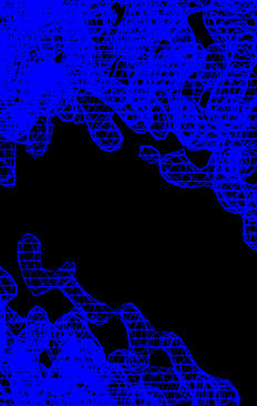
Electron density maps before and after solvent flipping are computed
with modified copies of the fourier_map.inp task file. Note
that when making the map using the density modified phases the
reflection array produced by the density modification is used rather
than the native amplitudes. This reflection array contains estimated
amplitudes (and phases) for any missing reflections, these
reconstructed reflections can help improve the map, especially for
missing low resolution data.
      cns_solve < fourier_map_mad.inp > fourier_map_mad.out  [22 seconds]
      cns_solve < fourier_map_dm.inp > fourier_map_dm.out    [23 seconds]
If you have mapman installed, you can use the command
map_to_omap *.map
to convert the CNS maps to a format which can be read into O.
The refined heavy-atom positions in mad_phase2.sdb (see previous tutorial) are converted to a PDB file for use in O.
cns_solve < sdb_to_pdb.inp > sdb_to_pdb.out [< 1 second]
In O, enter @omac to read in the maps and the heavy-atom
coordinates.
|
|
| Experimental MAD phased map | After solvent flipping |