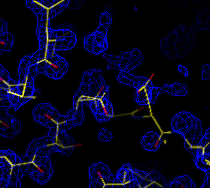
A discrepancy is seen between the model and density around residue B117.
The free R-value of the model has now dropped to 32% (the ytterbiums contribute significantly to the scattering). Inspection of the electron density map followed by manual rebuilding is now performed to improve the model. A cross-validated, sigma-A weighted 2Fo-Fc map is calculated. Inspection of this map will help locate areas of the model which are in error. It would also be helpful to look at a difference map (at both positive and negative contour) at the same time. Here the map is calculated using the CNS task file model_map_2fofc.inp:
cns_solve < model_map_2fofc.inp > model_map_2fofc.out [1 minute]
If you have mapman installed, you can use the command
map_to_omap *.map
to convert the CNS maps to a format which can be read into
O. In O, enter @omac to read in the
current model and map.
The map is in general very good - the density clearly matches the model. However, there is a region where there is an obvious difference between the model and the electron density:
 |
| Sigma-A weighted 2Fo-Fc map (at 1.5 sigma). A discrepancy is seen between the model and density around residue B117. |
In order to obtain less biased density for this region a simulated annealing omit map is calculated. We will omit the first 10 residues from molecule B (residues B109 to B118). Residues immediately surrounding these will also be omitted (this is done automatically in the CNS task file). A short simulated annealing refinement is performed to attempt to remove model bias to the missing region. The result is an electron density map. The CNS task file sa_omit_map.inp is used:
cns_solve < sa_omit_map.inp > sa_omit_map.out [13 minutes]
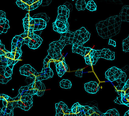
The map shows improved density for the correct placement of the N-terminal residues. There is a register shift of one residue resulting in a more open loop:
 |
| Sigma-A weighted 2Fo-Fc simulated annealing omit map (at 1.25 sigma). The correct trace for the N-terminal residues in molecule B are clearer. |
The model is manually rebuilt in this region resulting in a new set of coordinates. These coordinates are then used to make new CNS coordinate and molecular topology files for further refinement. Here the CNS task file generate_easy_reb.inp is used:
cns_solve < generate_easy_reb.inp > generate_easy_reb.out [2 seconds]
The refinement is started with simulated annealing, which will correct any errors introduced by the manual rebuilding and optimize the fit of the retraced region. As before a start temperature of 5000K is used. Here the CNS task file anneal_reb.inp is used:
cns_solve < anneal_reb.inp > anneal_reb.out [47 minutes]
At this point the free R-value is just below 31% (and the R-value is just below 28%). The model still might have some misplaced atoms (side chain atoms or small loops) but inspection of the maps suggest that the majority of the structure is correct. We therefore proceed with restrained individual B-factor refinement in preparation for automated water picking (see next section). The B-factor refinement is carried out with the CNS task file bindividual.inp:
cns_solve < bindividual.inp > bindividual.out [2 minutes]